Introduction
We have seen in the last post about graph signal processing and the Fourier transformation of graph data. In summary, transforming a 1D signal defined on graphs with \(n\) nodes (denoted as \(\mathbf{g} \in \mathbb{R}^n\)) requires the matrix of eigenvectors of the Laplacian matrix \(L = D - A\). Assuming that we have decomposed the Laplacian as \(L = U\Lambda U^T\), the transformation can be written as:
\[\hat{\mathbf{g}}[l] = {\bf u}_l^{T}{\bf g}\]where \(\mathbf{u}_l\) is the \(l\)-th column in \(U\).
Filtering operations are also defined in the frequency domain. Now following the notation from (Defferrard et al., 2016), the convolution operation between two signals \(x\) and \(y\) on graph \(G\) is defined as:
\[x *_{G}y = U((U^Tx)\odot(U^Ty)),\]where it transforms both \(x\) and \(y\) to the frequency domain (\(U^Tx\) and \(U^T y\)), perform the convolution operation (\((U^Tx)\odot(U^Ty)\)), and return to the original domain (\(U((U^Tx)\odot(U^Ty))\)). Note that from the convolution theorem, element-wise multiplications in the frequency domain is the same as convolution on the original domain. In the previous post, \(U^Ty\) is analogous to the filtering operation \(h(\Lambda)\), and \(x\) to \(\mathbf{g}\) (or vice versa, actually).
However, the most widely used form of graph convolution (GCN model from Kipf & Welling) is still far from the above formulation. Between GCN and the classical graph Fourier transform, an intermediate work (Defferrard et al., 2016) has been proposed to reduce the complexity, and thus proposing a learnable graph learning model that later inspired (Defferrard et al., 2016). We will try to understand the thought behind (Defferrard et al., 2016) and perform some analysis using an experiment proposed by (Alon & Yahav, 2021).
ChebConv
Firstly, let us assume that we are interested in learning a filter (or graph neural network) on a given graph \(G\). Based on the description above, the straightforward approach of modeling \(h(\Lambda)\) is just making the vector \(x \in \mathbb{R}^n\) learnable. This introduces a total of \(n\) parameters (this is the non-parametric filter in ChebConv).
Two modifications from non-parametric filters
The first modification of ChebConv is to reduce the number of parameters from \(n\) to \(K\) (of course, \(K < n\)) by setting \(h(\Lambda)\) as a polynomial filter. That is, the filter \(h(\Lambda)\) is now expressed with respect to polynomial basis (which is literally polynomials of \(\Lambda\): \(I\), \(\Lambda\), \(\Lambda^2\), \(\cdots\)) with coefficients \(\theta_k\):
\[h(\Lambda) = \sum_{k=0}^{K-1}\theta_k \Lambda^k.\]Putting this version of the filter to process the graph signal \(x\):
\[\mathbf{h}(\Lambda)x = U (\sum_{k=0}^{K-1}\theta_k \Lambda^k) U^T x = \sum_{k=0}^{K-1}\theta_k (U\Lambda^kU^T)x = \sum_{k=0}^{K-1}\theta_k L^kx\](Note that \(UU^T = I\)).
Now the filter is \(K\)-localized, according to [2]. Intuitively, assuming the Laplacian is \(L = D-A\), notice that \(L^{K-1} = (D-A)^{K-1}\) contains \(I\) to \(A^{K-1}\), suggesting that the new signal \(\mathbf{h}(\Lambda)x\) contains information from each node to its \((K-1)\)-hop neighbor.
The second modification is to use the Chebyshev polynomials instead of the polynomial basis. This has a number of advantages, such as the use of orthogonal basis, and more importantly, increase in efficiency since the basis can be recursively defined:
\[\mathbf{h}(\Lambda) = \sum_{k=0}^{K-1} \theta_k T_k(\Lambda)\](ChebConv replaces \(\Lambda\) with the normalized version \(\tilde{\Lambda}\), but we will not consider this here).
Implications of the ChebConv formulation
As mentioned above, the main implication of this version of graph filtering is that now the convolution affects a local neighborhood of each node, determined by the number of basis used. We will see this effect directly using the NEIGHBORSMATCH problem (Alon & Yahav, 2021).
Observing the locality effect
The NEIGHBORSMATCH problem
Proposed by (Alon & Yahav, 2021), the NEIGHBORSMATCH problem is a task involving synthetically generated graphs. The intention of the problem is to create a task with a specific problem radius (i.e., the required range of interaction between a node and its neighbors for the model to solve the problem). It generates a number of synthetically generated graphs with problem radius \(r\), and a graph neural networks (GNNs) is trained to solve the task. If the GNN has less than \(r\) layers, it cannot solve the problem whatsoever.
Our modification
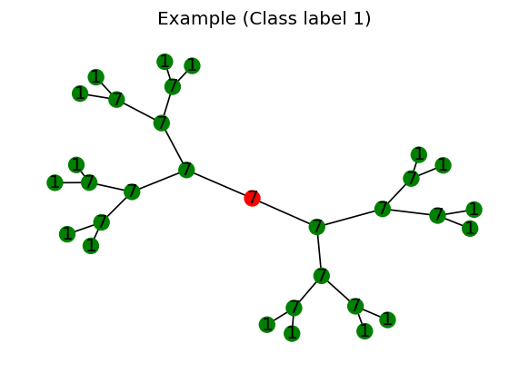
In our case, we slightly modify the NEIGHBORSMATCH problem to a more simpler configuration. Consider a synthetically generated graph below:

[Appendix 1: Source code for the simplified NEIGHBORSMATCH] [Appendix 2: Code for generation] [Appendix 3: Code for visualizing]
Figure 1 visualizes a single graph within the dataset generated from the code. These are some features of the graph and the dataset:
- The graph is a full binary tree, with the root node colored in red in the Figure.
- Each node is assigned with a randomply assigned integer, which serves as the node features (in implementation, the integer is encoded as a one-hot vector).
- The assigned integers of the leaf node is different with the rest of the nodes within the graph.
- The integers of the leaf node is defined as the class label of the root node.
- Consequently, the integer of the root node does not have any relationships with the actual class label.
Similar to the original version, given a dataset consisting of such graphs, we are interested in classifying the root node ‘directly’ by using a GNN model; that is, the GNN model is to compute the class probability of the root by aggregating the neighbor information w.r.t. the root node itself.
A direct consequence of this is that the GNN cannot solve the NEIGHBORSMATCH problem unless it has aggregated information from the leaf node to the root node.
Directly observing the effect of \(K\)
Here, we aim to observe the receptive field generated from the ChebConv using the modified NEIGHBOURSMATCH problem above. In the following experiment, we make a GNN model using exactly one ChebConv layer with a pre-defined value of \(K\). We try to observe whether our GNN model can solve this problem with different depths of the dataset.

[Appendix 4: Model code] [Appendix 5: Experiment code]
- We see in Figure 2 that for different values of depth for the NEIGHBORSMATCH dataset, ChebConv requires a localized filter that can at reach the leaf nodes. This is expected since the information crutial for solving the problem only exists at the feature vectors of the leaf node by design.
- Also, since the problem itself is very straightforward, the performance of the models for those that can solve is always near 1. This is despite the fact that we only used one layer of ChebConv without any non-linear actiavation functions.
- For the models that could not solve the problem, the performance degrades to a random classifier: The performance is always near \(\approx 1/(\text{num. of class})\).
Chance of redemption: Stacking layers
For ChebConv layers that does not have enough receptive field, we can still make the models solve the problem with a simple modification: stacking the layers. Since each convolutions aggregate information from the neighbors from the receptive field, stacking multiple convolutions will make the information travel more. This design choice is also highlighted in the next paper that we will cover (GCN).
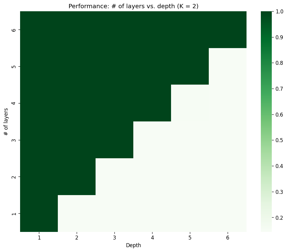
To see this effect, we will build several models using ChebConv layers, each with receptive field of \(K=2\). However, the task will be generated with varying depth values from 1 to 6 . In the first experiment (where we restricted ourselves to a one layer model), the model is bound to fail for depth greater than 1. In this experiment, we will attempt to stack layers for all depth values until the model can finally solve the problem.

[Appendix 6: Model code] [Appendix 7: Experiment log]
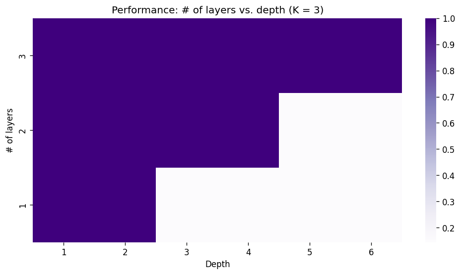
Here, we can see that stacking enough layers, the model will eventually be able to solve the task. Also notice that for the cases where the model fails, the performance is roughly \(1/(\text{num. of classes})\), indicating that the model is basically a random classifier. Let’s look at an another case where we stack ChebConv layers with \(K=3\):

[Appendix 8: Experiment log]
As expected, the depth that the model can solve now increases twice as fast per layer compared to the case when \(K=2\). Note that there are no benefits of stacking layers for \(K=1\) for solving NEIGHBORSMATCH as it only learns filters of itself (remember the first term of the Chebyshev polynomial is the identity matrix \(I\)) and does not take neighbor nodes into consideration.
Conclusions
We have observed the main idea of ChebConv, along with its interpretation in terms of receptive field. Running various experiments on the NEIGHBORSMATCH problem, we were able to directly observe the effect of \(K\) on the solvability of the task, which is designed to be solved with a model that can cover the task’s problem radius.
Appendix
Appendix 1
import torch
import torch_geometric
from torch_geometric.data import Data
from torch.nn import functional as F
from sklearn.model_selection import train_test_split
import numpy as np
import random

"""
Based on the original implementation of the NEIGHBORSMATCH dataset.
Original implementation: https://github.com/tech-srl/bottleneck
Alon & Yahav, "ON THE BOTTLENECK OF GRAPH NEURAL NETWORKS AND ITS PRACTICAL IMPLICATIONS", ICLR 2021
"""

class TreeDataset:
    def __init__(self, depth: int = 5, num_of_class: int = 7):
        super(TreeDataset, self).__init__()
        self.depth = depth
        self.num_nodes, self.edges, self.leaf_indices = self._create_blank_tree()
        self.criterion = F.cross_entropy
        self.num_of_class = num_of_class
        self.feature_constructor = torch.eye(self.num_of_class + 1)

    def add_child_edges(self, cur_node, max_node):
        edges = []
        leaf_indices = []
        stack = [(cur_node, max_node)]
        while stack:
            cur_node, max_node = stack.pop()
            if cur_node == max_node:
                leaf_indices.append(cur_node)
                continue
            left_child = cur_node + 1
            right_child = cur_node + 1 + ((max_node - cur_node) // 2)
            edges.extend(
                (
                    [left_child, cur_node],
                    [right_child, cur_node],
                    [cur_node, left_child],
                    [cur_node, right_child],
                )
            )
            stack.append((right_child, max_node))
            stack.append((left_child, right_child - 1))
        return edges, leaf_indices

    def _create_blank_tree(self):
        max_node_id = 2 ** (self.depth + 1) - 2
        edges, leaf_indices = self.add_child_edges(cur_node=0, max_node=max_node_id)
        return max_node_id + 1, edges, leaf_indices

    def create_blank_tree(self, add_self_loops=False):
        edge_index = torch.tensor(self.edges).t()
        if add_self_loops:
            edge_index, _ = torch_geometric.utils.add_remaining_self_loops(
                edge_index=edge_index,
            )
        return edge_index

    def generate_data(self, train_fraction, num_examples: int = 20000):
        data_list = []

        for _ in range(num_examples):
            edge_index = self.create_blank_tree(add_self_loops=False)
            nodes, label = self.get_nodes_features_and_labels()
            data_list.append(
                Data(x=nodes, edge_index=edge_index, y=label)
            )

        X_train, X_test = train_test_split(
            data_list,
            train_size=train_fraction,
            shuffle=True,
            stratify=[data.y for data in data_list],
        )

        return X_train, X_test

    def get_nodes_features_and_labels(self):
        label = random.randint(0, self.num_of_class - 1)
        feature_ind = torch.LongTensor([-1] * self.num_nodes)
        feature_ind[self.leaf_indices] = label

        return torch.Tensor(self.feature_constructor[feature_ind]), label
Appendix 2
"""
Code for generating the dataset
Modify the depth, num_of_class, and train_fraction for your need
"""
tree = TreeDataset(depth=4, num_of_class=7)
X_train, X_test = tree.generate_data(train_fraction=0.8)
Appendix 3
"""
Code for visualizing one of the dataset.
"""
import networkx as nx
from torch_geometric.utils import to_networkx
import matplotlib.pyplot as plt

ind = 0 # Index of the graph to visulaize
tree_nx = to_networkx(X_train[ind], to_undirected=True) # Need networkx for this
# Node features
labeldict = {i: torch.argmax(X_train[ind].x[i]).item() for i in range(X_train[ind].x.shape[0])}
color = ['r'] + ['g'] * (X_train[ind].x.shape[0] - 1) # Only the root node is colored as red

# Draw via networkx
plt.figure(dpi = 120)
plt.title(f"Example (Class label {X_train[ind].y})")
nx.draw(tree_nx, labels = labeldict, with_labels = True, node_color = color, node_size = 100)
Appendix 4
from torch_geometric.nn import ChebConv


class GNN(torch.nn.Module):
    def __init__(self, in_channels, out_channels, K, num_layers):
        super().__init__()

        self.convs = torch.nn.ModuleList()
        for _ in range(num_layers - 1):
            self.convs.append(
                ChebConv(in_channels=in_channels, out_channels=in_channels, K=K)
            )
        self.convs.append(
            ChebConv(in_channels=in_channels, out_channels=out_channels, K=K)
        )

    def forward(self, x, edge_index, batch):
        num_nodes = int(x.shape[0] / len(batch.unique()))
        for conv in self.convs:
            x = conv(x=x, edge_index=edge_index, batch=batch)
        root_index = torch.LongTensor(list(range(0, len(batch), num_nodes)))
        return x[root_index]
Appendix 5
import torch
import torch.nn.functional as F
from torch_geometric.nn import ChebConv
from torch_geometric.loader import DataLoader
from itertools import product


class Experiment:
    def __init__(self, num_layers, K, depth, num_of_class):
        self.device = torch.device("cuda" if torch.cuda.is_available() else "cpu")
        self.K = K
        self.depth = depth
        self.train_loader, self.test_loader = self.prepare_dataset(depth, num_of_class)
        self.model = GNN(
            in_channels=self.in_channels,
            out_channels=self.out_channels,
            K=K,
            num_layers=num_layers,
        ).to(self.device)
        self.optimizer = torch.optim.Adam(self.model.parameters(), lr=0.0001)
        self.epochs = 8

    def make_data(self, depth, num_of_class):
        tree = TreeDataset(depth=depth, num_of_class=7)
        self.in_channels = tree.num_of_class + 1
        self.out_channels = tree.num_of_class
        return tree.generate_data(train_fraction=0.8)

    def prepare_dataset(self, depth, num_of_class):
        X_train, X_test = self.make_data(depth, num_of_class)
        train_loader = DataLoader(X_train, batch_size=16, shuffle=True)
        test_loader = DataLoader(X_test, batch_size=len(X_test))
        return train_loader, test_loader

    def train(self):
        self.model.train()
        total_loss = 0
        for data in self.train_loader:
            data = data.to(self.device)
            self.optimizer.zero_grad()
            out = self.model(x=data.x, edge_index=data.edge_index, batch=data.batch)
            loss = F.cross_entropy(out, data.y)
            loss.backward()
            self.optimizer.step()
            total_loss += float(loss) * data.num_graphs
        return total_loss / len(self.train_loader.dataset)

    @torch.no_grad()
    def test(self, loader):
        self.model.eval()
        total_correct = 0
        for data in loader:
            data = data.to(self.device)
            pred = torch.argmax(
                self.model(x=data.x, edge_index=data.edge_index, batch=data.batch),
                dim=1,
            )
            total_correct += int((pred == data.y).sum())
        return total_correct / len(loader.dataset)

    def run_experiment(self):
        for _ in range(self.epochs):
            loss = self.train()
            train_acc = self.test(self.train_loader)
            test_acc = self.test(self.test_loader)
        return test_acc

"""
Run the actual experiment
"""
performance_heatmap = np.zeros((8,8))

for K, depth in product(range(2, 8), range(1, 7)):
    perf = Experiment(num_layers=1, K=K, depth=depth, num_of_class=7).run_experiment()
    performance_heatmap[K][depth] = perf
    print(f"K: {K}, depth: {depth}, performance: {perf}")


>>>
K: 2, depth: 1, performance: 1.0
K: 2, depth: 2, performance: 0.144
K: 2, depth: 3, performance: 0.1445
K: 2, depth: 4, performance: 0.14725
K: 2, depth: 5, performance: 0.14325
K: 2, depth: 6, performance: 0.14725
K: 3, depth: 1, performance: 1.0
K: 3, depth: 2, performance: 1.0
K: 3, depth: 3, performance: 0.14875
K: 3, depth: 4, performance: 0.14425
K: 3, depth: 5, performance: 0.147
K: 3, depth: 6, performance: 0.1425
K: 4, depth: 1, performance: 1.0
K: 4, depth: 2, performance: 1.0
K: 4, depth: 3, performance: 1.0
K: 4, depth: 4, performance: 0.1455
K: 4, depth: 5, performance: 0.1475
K: 4, depth: 6, performance: 0.14625
K: 5, depth: 1, performance: 1.0
K: 5, depth: 2, performance: 1.0
K: 5, depth: 3, performance: 1.0
K: 5, depth: 4, performance: 1.0
K: 5, depth: 5, performance: 0.14825
K: 5, depth: 6, performance: 0.1445
K: 6, depth: 1, performance: 1.0
K: 6, depth: 2, performance: 1.0
K: 6, depth: 3, performance: 1.0
K: 6, depth: 4, performance: 1.0
K: 6, depth: 5, performance: 1.0
K: 6, depth: 6, performance: 0.14525
K: 7, depth: 1, performance: 1.0
K: 7, depth: 2, performance: 1.0
K: 7, depth: 3, performance: 1.0
K: 7, depth: 4, performance: 1.0
K: 7, depth: 5, performance: 1.0
K: 7, depth: 6, performance: 1.0
Appendix 6
class GNN_new(torch.nn.Module):
    def __init__(self, in_channels, out_channels, K, num_layers):
        super().__init__()
        self.num_layers =  num_layers
        self.convs = torch.nn.ModuleList()

        for i in range(num_layers):
            if i < num_layers - 1:
                self.convs.append(ChebConv(in_channels=in_channels, out_channels=in_channels, K=K))
            else:
                self.convs.append(ChebConv(in_channels=in_channels, out_channels=out_channels, K=K))

    def forward(self, x, edge_index, batch):
        num_nodes = int(x.shape[0] / len(batch.unique()))
        for i in range(self.num_layers):
            x = self.convs[i](x, edge_index)
        root_index = torch.LongTensor(list(range(0, len(batch), num_nodes)))
        return x[root_index, :]
Appendix 7
Num_layers: 1, depth: 1, performance: 1.0
Num_layers: 1, depth: 2, performance: 0.146
Num_layers: 1, depth: 3, performance: 0.14475
Num_layers: 1, depth: 4, performance: 0.14725
Num_layers: 1, depth: 5, performance: 0.14525
Num_layers: 1, depth: 6, performance: 0.1445
Num_layers: 2, depth: 1, performance: 1.0
Num_layers: 2, depth: 2, performance: 1.0
Num_layers: 2, depth: 3, performance: 0.14525
Num_layers: 2, depth: 4, performance: 0.14525
Num_layers: 2, depth: 5, performance: 0.14425
Num_layers: 2, depth: 6, performance: 0.1465
Num_layers: 3, depth: 1, performance: 1.0
Num_layers: 3, depth: 2, performance: 1.0
Num_layers: 3, depth: 3, performance: 1.0
Num_layers: 3, depth: 4, performance: 0.1455
Num_layers: 3, depth: 5, performance: 0.145
Num_layers: 3, depth: 6, performance: 0.1445
Num_layers: 4, depth: 1, performance: 1.0
Num_layers: 4, depth: 2, performance: 1.0
Num_layers: 4, depth: 3, performance: 1.0
Num_layers: 4, depth: 4, performance: 1.0
Num_layers: 4, depth: 5, performance: 0.1485
Num_layers: 4, depth: 6, performance: 0.14475
Num_layers: 5, depth: 1, performance: 1.0
Num_layers: 5, depth: 2, performance: 1.0
Num_layers: 5, depth: 3, performance: 1.0
Num_layers: 5, depth: 4, performance: 1.0
Num_layers: 5, depth: 5, performance: 1.0
Num_layers: 5, depth: 6, performance: 0.14425
Num_layers: 6, depth: 1, performance: 1.0
Num_layers: 6, depth: 2, performance: 1.0
Num_layers: 6, depth: 3, performance: 1.0
Num_layers: 6, depth: 4, performance: 1.0
Num_layers: 6, depth: 5, performance: 1.0
Num_layers: 6, depth: 6, performance: 1.0
Appendix 8
Num_layers: 1, depth: 1, performance: 1.0
Num_layers: 1, depth: 2, performance: 1.0
Num_layers: 1, depth: 3, performance: 0.145
Num_layers: 1, depth: 4, performance: 0.14575
Num_layers: 1, depth: 5, performance: 0.14675
Num_layers: 1, depth: 6, performance: 0.14625
Num_layers: 2, depth: 1, performance: 1.0
Num_layers: 2, depth: 2, performance: 1.0
Num_layers: 2, depth: 3, performance: 1.0
Num_layers: 2, depth: 4, performance: 1.0
Num_layers: 2, depth: 5, performance: 0.1445
Num_layers: 2, depth: 6, performance: 0.145
Num_layers: 3, depth: 1, performance: 1.0
Num_layers: 3, depth: 2, performance: 1.0
Num_layers: 3, depth: 3, performance: 1.0
Num_layers: 3, depth: 4, performance: 1.0
Num_layers: 3, depth: 5, performance: 1.0
Num_layers: 3, depth: 6, performance: 1.0