Introduction
In graph signal processing (GSP), graph data is analyzed in the Fourier domain. Although Fourier analysis itself is already well-known on other types of data, extending the Fourier transform for analysis on graph data is quite interesting and worth diving into.
This post concerns the basic idea of GSP and further investigates its application with the Cora dataset.
Notations
For ease of description, let us define some notations and assumptions before moving on.
Basic graph notations
- Let us assume a graph \(G=(V, E)\) is given, where \(V\) is the set of nodes and \(E\).
- The number of nodes in the graph is \(n\).
- It makes life simple if we think of each node \(i \in V\) also as natural numbers (\(i = 1, \cdots, n\)).
- The adjacency matrix is denoted as \(A\), and the degree matrix as \(D = diag(d_1, \cdots, d_n)\) where \(d_i = \sum_{j=1}^n A_{ij}\).
Graph signals
- For each node \(i \in V\), a single scalar is assigned as the signal of the node. Its basically the same as defining the node feature matrix, where the dimension of the features is one.
- The graph signal is represented as a \(n\)-dimensional vector \({\bf g} \in \mathbb{R}^{n}\). Making our notations pytorch-like, the signal for node \(i\) is denoted as \({\bf g}[i] \in \mathbb{R}\) (But here \(i\) starts at 1, not zero).
Extension of Fourier transform to graphs
1D Fourier transform
Fourier transforms enables us to view the given data from the original domain (such as time) to the frequency domain. To apply such transformations to graph signals (data defined on graphs), we need to first generalize the Fourier transformation itself. This insight is nicely described in (Shuman et al., 2013), which we will follow also.
The most frequent (no pun intended) equation that you might have encountered when looking up for Fourier transformation would be the following:
where the function \(f\) defined on the (probably) time domain (i.e., \(t\)) is transformed into a function \(\hat{f}\) defined on the frequency domain (i.e., \(\zeta\)). The interpretation of the integral itself is beautifully described by 3Blue1Brown (link).
In more general terms, the Fourier transformation can be thought of as the inner product between the original function and the eigenfunctions of the Laplace operator. Concretely,
\[\hat{f}(\zeta) = <f, e^{2\pi i\zeta i}>,\]and you can see the first equation naturally aligns with the general definition of Fourier transform. Eq. (2) in (Shuman et al., 2013) also shows that \(e^{2\pi i \zeta i}\) is indeed the eigenfunction of the Laplace operator in 1D.
Graph fourier transform
This generalized definition provides the way to extend the Fourier transformation to graph data. By reminding that the graph data is a discrete data that are represented as vectors rather than functions, the extension of Fourier transform is now clear : 1) Get the eigenvectors of the Laplacian matrix 2) Inner product with the original graph signal.
More concretely, the transformed graph signal is described as:
\[\hat{\mathbf{g}}[l] = <{\bf g}, {\bf u}_l>,\]where \({\bf u}_l\) is the eigvenvector corresponding to the \(l\)-th lowest eigenvalue of the Laplacian matrix (\(l = 1, \cdots, n\)). Notice that the domain has shifted from \(i\) to \(l\).
This implies several things:
- The Laplacian matrix is conceptually equivalent as the Laplace operator: (Shuman et al., 2013) provides an intuitive explanation by introducing concepts from discrete calculus.
- We need to perform eigendecomposition for the Laplacian matrix for this to happen: We need the eigenvectors \({\bf u}_l\).
- The inner product is now vector multiplication between vectors:
- Or, in vector form:
Eigendecomposing SBMs
To see what the eigenvectors of the graph Laplacian is, lets directly compute such vectors by using an intuitive example. Perhaps the best example to illustrate is stochastic block models (SBMs), which is a graph generative model where the user can control simple community structures genertated from the model.
Two pieces of information is required for the SBM model to generate graphs with \(c\) number of communities: A vector that defines the number of nodes to be included in each community, and a symmetric matrix indicating the edge probability between (or within) communities.
The code below shows one example of an SBM model generated by pytorch geometric, with the help of the networkx package for visualization:
# Generate SBM graph with Pytorch Geometric
import torch_geometric as pyg
from torch_geometric.data import Data
from torch_geometric.utils import stochastic_blockmodel_graph as sbm
from torch_geometric.utils import to_networkx
import networkx as nx

block_sizes = [40, 60]  # Two communities
node_color = ["red"] * 40 + ["blue"] * 60  # Set node colors for drawing
edge_probs = [[0.2, 0.005], [0.005, 0.2]]  # Symmetric since our graph is undirected

# Graph data in PyG is represented as a torch_geometric.data.Data object
sbm_torch = Data(
    edge_index=sbm(block_sizes=block_sizes, edge_probs=edge_probs),
    num_nodes=sum(block_sizes),
)

# To visualize, move from torch_geometric.data.Data to networkx.Graph object
sbm_torch = to_networkx(sbm_torch, to_undirected=True)
nx.draw(sbm_torch, node_size=50, node_color=node_color)
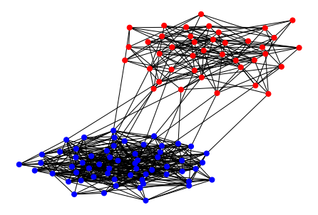
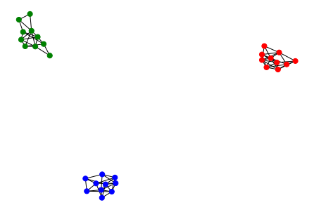
In Figure 1, the probability of an edge existing between different communities (color coded in blue and red, respectively) is set to 0.005, while the probability within the same community is set to 0.2. Note that the edges are independently generated. If we set the probability between different community to zero, graphs such as in Figure 2 will be generated.
We will use the following quite dramatic but managable graph for decomposition:

The eigendecomposition of the unnormalized graph Laplacian \(L = D-A\) is easilty computed by modern libraries, such as numpy or pytorch. The values of the sorted eigenvalues are as follows:

We can clearly see that three eigenvalues are at zero, indicating that there are three very distinct community structures (i.e., connected components) within the graph structure. The smallest eigenvalues (frequencies) correspond to number of connected components, since connected components is the most ‘macro’ view when looking at the graph structure. This is analogous to the Fourier series expansion of a periodic function. Roughly speaking, the Fourier series expansion can be thought of re-expressing a function with sine and cosine basis:
\[f(x) = a_0 + \sum_{n}^{\infty}(a_n \sin (\omega_nx) + b_n \cos (\omega_nx)),\]and the ‘lowest frequency’ sine and cosines inside the summation have the ‘widest’ valleys (or the ‘macro’ view since they are responsible of describing the large-scale characteristics).
We can them anticipate the eigenvalues when we slightly modify the graph (see Figure 4):


Now, the number of zero eigenvalues in Figure 6 becomes one, since the graph now has one connected component. However we can still see that the second and third lowest values are still quite near zero.
It is also worth illustrating the eigenvectors itself. Following conventional notiations, lets say that the Laplacian matrix \(L\) is decomposed into \(L = U \Lambda U^{T}\), where the diagonal matirx \(\Lambda\) contains the (ordered) eigenvalues and \(U\) contains the eigenvectors:
\[U = \begin{bmatrix} \vert & &\vert \\ {\bf u}_1 & \cdots & {\bf u}_{n} \\ \vert & &\vert \end{bmatrix}\]Lets straight up visualize \(U\).

Here, we can see the different modes of the graph signals, which are combined together to form the original graph signals. In the left-most column (\({\bf u}_1\)), the values all have the same values. This eigenvector corresponds to the lowest eigenvalue (which is zero), and the same values indicate the ‘one connected component’ information.
However, the eigenvector right next to it (\({\bf u}_2\), corresponding to the second-lowest eigenvalue) still shows the three community structures present in the graph. To be more explicit, lets plot \({\bf u}_1\):

In short, assuming that the graph has only one connected component, \({\bf u}_1\) encodes the community structure of the graph. This is actually the main idea behind spectral clustering (Luxberg, 2007).
Low-pass filtering Cora
Regarding graph signal processing and Fourier transform, the paper (NT & Maehara, 2019) introduces a straightforward experiment on the Cora dataset (Yang et al., 2016) (Specifically, section 3).
The experiment procedure in (NT & Maehara, 2019)
Denoting the feature matrix of Cora as \(X \in \mathbb{R}^{2703 \times 1433}\) and given an index \(k \in [1, 2703]\), this is the experiment procedure:
- Compute the Fourier basis \(U\) by eigendecomposing the graph Laplacian.
- Add Gaussian noise to the feature matrix: \(X \leftarrow X + \mathcal{N}(0, \sigma^2)\)
- Compute the lowest \(k\)-frequency component: \(X_k \leftarrow U[:k]^T X\)
- Reconstruct the features: \(\tilde{X}_k = U[:k] X_k\)
- Train an MLP on \(\tilde{X}_k\) for semi-supervised node classification.
We attempt to reproduce the results and make some discussions and interpretations. In our case, we use the unnormalized graph Laplacian \(L = D-A\) as opposed to the symmetrically normalized version \(L_{norm} = D^{-1/2}AD^{-1/2}\). We also discard step 2 since we are not interested in robustness to noise.
In theory
In theory, this is the same as low-pass filtering on the feature matrix \(X\). Rewriting in terms of (Shuman et al., 2013) (Look at Section III-A for more details), the procedure is the same as defining a filtering function \({\bf h}\), where in
\[{\bf h}(L) = U \begin{bmatrix} h(\lambda_1) & & {\bf 0}\\ & \ddots & \\ {\bf 0} & & h(\lambda_n) \end{bmatrix} U^T,\]the function \(h\) is defind as:
\[h(\lambda_i) = \begin{cases} 1 & \text{if}\ i \leq k \\ 0, & \text{otherwise} \end{cases}.\]In summary, the whole process can be described as
\[\mathbf{h}(L)X = U \mathbf{h}(\Lambda)U^T X,\]where it transforms the feature matrix \(X\) to the frequency domain (\(U^T X\)), modify the signal by the function \(h\) (\(\mathbf{h}(\Lambda)U^T X\)), and return to the original domain (\(U \mathbf{h}(\Lambda)U^T X\)).
Focusing on \(h(\lambda_i)\), it basically cuts off higher frequency signals (remind that the frequencies are determined by the graph structure) where the cutoff is at the \(k\)-th lowest frequency value. It just leaves the Fourier basis that are equal or below the \(k\)-th frequency.
Our experiment
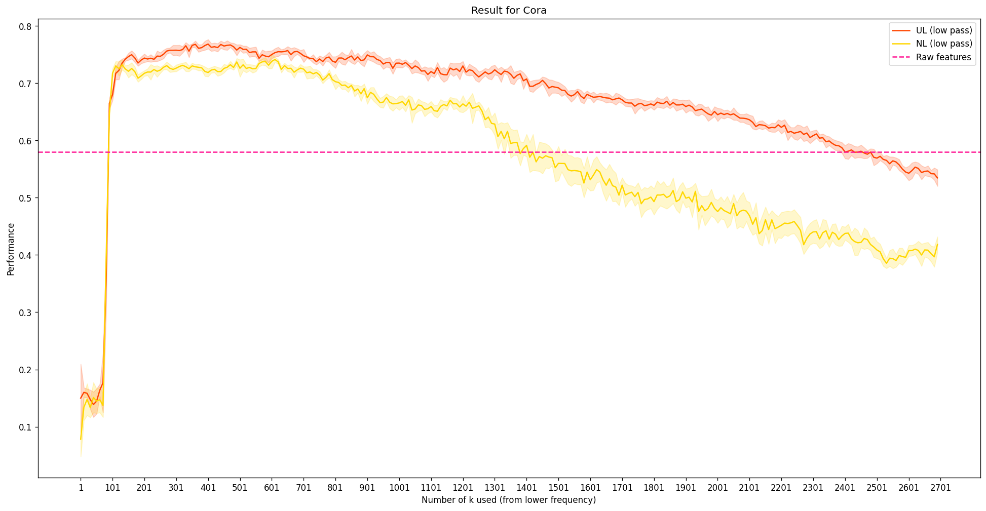
This is the experimental result to reprocude (NT & Maehara, 2019), where
- A 2 layer MLP was trained with early stopping.
- Same semi-supervised node classification setting as in (Yang et al., 2016).
- 10 independent trials, plotting the average values in a solid line, alongside the one standard deviation.
- We plot the results alongside with the performance of an MLP with the same configurations using the original feature matrix \(X\) (pink dotted line).
- UL stands for unnormalized Laplacian (red line), NL stands for symmetrically normalized Laplacian (yellow line)

So, there are several things that are noticeable here:
- As expected, the performance is not so great at the extreme low end: There are simply not enough information for the MLP to get going.
- The peak performance happens near \(k\approx400\), even exceeding the case with using the original features. The value \(400\) is still quite a low value, considering that \(k\) can be up to 2703: This implies that the dataset itself benefits from low-frequency structure information. Such tendency aligns with the previous blog post, where assuming that nodes that are connected will probabily have similar labels helps solve node classification on Cora. Remind that locally, low-frequency means that the values between connected nodes does not change much.
- However, it seems quite weird that the performance does not seem to exactly recover the pink dotted line as we still continue to increase \(k\) near 2703. This issue will probably be linked with the computation error during the eigendecomposition. To show this, we directly calculate the difference bewteen \(X\) and \(U U^T X\): In theory, this is 0. In code, sadly, this is not the case:
import torch
from torch.linalg import eig

L, U = eig(laplace)
L_norm, U_norm = eig(laplace_norm)

# torch.dist: https://pytorch.org/docs/stable/generated/torch.dist.html
torch.dist((U @ U.T).real @ data.x, data.x)

>> tensor(114.4097)

torch.dist((U_norm @ U_norm.T).real @ data.x, data.x)

>> tensor(101.5464)
Conclusion
In this blog post, we have looked at the extension of Fouirer transformation in graph data as the core idea of graph signal processing. The re-representation of the graph in the frequency doman has quite straighforward interpretations, and we have also seen that the basis corresponding to the low frequency directly shows the macro-level structure. Expanding on the interpretation, we reprocude the experimental result in (NT & Maehara, 2019), which directly show that the low-frequency features are vital in the semi-supervised classification for Cora.
Appendix
This is just out of curiosity, how about \(\mathcal{L}X\) instead of \(X\)?
Here, the filter function is defined as
\[h'(\lambda_i) = \begin{cases} \lambda_i, & \text{if}\ i \leq k \\ 0, & \text{otherwise} \end{cases},\]where in this version the filter actually preserves the frequency of the Laplacian.
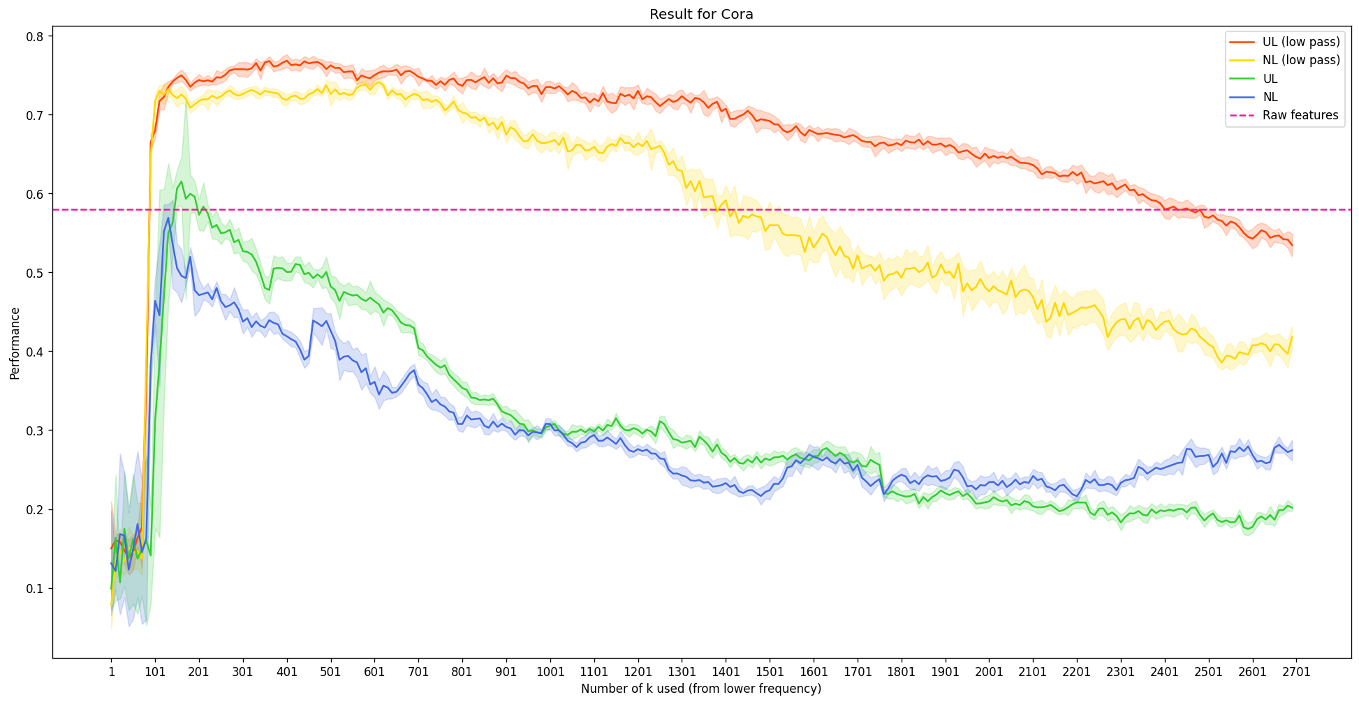
For brevity, we label different configurations as follows:
| Unnormalized Laplacian | Sym. norm. Laplacian | |
|---|---|---|
| \(h\) | UL (low pass) | NL (low pass) |
| \(h\)’ | UL | NL |
The expanded experimental results are as follows:

- Overall, the performance degenerates when we use some form of \(\mathcal{L}X\) instead of \(X\), although the tendency for different \(k\) still remains the same. Considering the unnnormalized Laplaican, \(\mathcal{L} = D-A\), the minus sign in front of the adjacency matrix suggest that we are not actually aggregating the neighbor information; rather, we are emphasizing the difference. It shows that this is a poor representation of \(X\) to solve this task.
- For the case where we use the symmetrically normalized Laplacian matrix, it is the only configuration that shows that the performace increases as we add more high frequency information (blue line). There can be several explanations for this:
- The high frequency information does have performance benefits for some limited cases
- The computation error from the eigendecomposition is less dominant and is therefore the reason of the performance increase
, which will be an interesting topic for future investigation.