Introduction

In the current deep learning era that we live in, we now have various models that are widely used not only in research but also real-world problem solving in other data types such as image and natural languages: ResNet, YOLO, BERT, GPT, to name a few. The equivalent model in the field of graph data is perhaps the GCN model (Graph Convolutional Networks) (Kipf & Welling, 2017).

GCN continues the effort made in ChebConv (Defferrard et al., 2016) in trying to build an efficient yet effective graph learning model, based on the framework of graph signal processing. Although not as commonly used but still well-known, SGC (Simple Graph Convolution) (Wu et al., 2019) proposes an even simpler model on top of GCN, resulting in the most straightforward model to interpret out of the three models. In this post, we will attempt to comprehensively compare the three models in terms of efficiency.

Architecture of three models

ChebConv

As mentioned, GCN starts from the ChebConv model. First, let us define several concepts and notations:

• A graph \(G\) with the set of nodes \(V\) and edges \(E \subseteq V \times V\) is described as \(G = (V, E)\).
• Let us assume the graph is unweighted and undirected.
• The graph structure can be represented as a symmetric square matrix \(A \in \{0,1\}^{V \times V}\), where \(A_{ij} = 1\) iff \((i,j) \in E\).
• The degree matrix \(D\) is a diagonal matrix, where \(D_{ii}\) is the degree of node \(i\), and zero elsewhere.
• The (normalized) Laplacian matrix of \(G\) is denoted as \(L = I - D^{-1/2} A D^{-1/2}\). In GCN, we use a normalized version of the Laplacian: \(\tilde{L} = \dfrac{2}{\lambda_{\max}}L - I\), where the eigenvalues of \(\tilde{L}\) are normalized to the range of \([-1, 1]\).

Then, the ChebConv layer can be described as:

, where \(T_k\) is the \(k\)-th basis function of the Chebyshev expansion and \(\theta_k\)’s are learnable parameters.

Formulation of GCN

Building upon Chebconv, GCN simplifies the convolution by only using the first two terms:

, and instead compensate by stacking multiple layers. Further approximating \(\lambda_{\max} = 2\), we can modify to:

Furthermore, we can set $\theta_0 = -\theta_1 = \theta$ to reduce the number of parameters:

Finally, using the renormalization trick to keep the range of eigenvalues within \([0,1]\), we are left the following convolution layer:

, where \(\Theta \in \mathbb{R}^{C \times d}\) is a learnable matrix which maps the \(C\)-dimensional convoluted signal to a \(d\)-dimensional representation. Denoting \(\sigma\) as some non-linear activation function (e.g., ReLU) and \(\bar{A} = \tilde{D}^{-1/2}A\tilde{D}^{-1/2}\) for simplicity, stacking \(L\) layers of the convolution results in the following model architecture (assuming we are solving node classification):

Here, the set of parameter matrices \(\mathbf{\Theta} = \{\Theta_1, \cdots ,\Theta_L\}\) are learned using gradient descent.

Formulation of SGC

As the name suggests, SGC aims to simplify GCNs even further. Starting from the original equation of GCN above, they remove most of the non-linearity in the GCN model:

Removing the non-linearities further enables to reduce all parameter matrices to just one, as we can just model compositions of multiple linear transformations as a single linear transformation:

Analysis of efficiency

Here, we aim to analyze the efficiency of the three models. Specifically, the model configuration is made as follows to ensure the receptive field remains the same:

• ChebConv: 1 layer model with \(K=2,3,4,5\).

• GCN: $L$ layer model with \(L=1,2,3,4\). The equation below shows the case when \(L=2\).

• SGC: 1 layer model with \(L=1,2,3,4\). The equation below shows the case when \(L=2\).

For the implementation, we will use pytorch with pytorch geometric as the main library, and the code for the model architecture is as follows:

• ChebConv

    import torch
    from torch_geometric.nn import ChebConv
      
    class GNN_Cheb(torch.nn.Module):
        def __init__(self, in_channels: int, K: int, out_channels: int = 7):
            super().__init__()
      
            self.convs = ChebConv(in_channels=in_channels, out_channels=in_channels, K=K)
      
        def forward(self, data):
            x, edge_index = data.x, data.edge_index
            x = self.convs(x=x, edge_index=edge_index)
            return x
  

• GCN

    import torch
    from torch_geometric.nn import GCNConv
      
    class GNN_GCN(torch.nn.Module):
        def __init__(
            self,
            in_channels: int,
            hidden_dim: int, # default: 128
            num_layers: int,
            out_channels: int = 7,
            cached: bool = False,
        ):
            super().__init__()
            self.convs = torch.nn.ModuleList()
            if num_layers > 1:
                self.convs.append(
                    GCNConv(
                        in_channels=in_channels,
                        out_channels=hidden_dim,
                        add_self_loops=True,
                        cached=cached,
                    )
                )
                for _ in range(num_layers - 2):
                    self.convs.append(
                        GCNConv(
                            in_channels=hidden_dim,
                            out_channels=hidden_dim,
                            add_self_loops=True,
                            cached=cached,
                        )
                    )
                self.convs.append(
                    GCNConv(
                        in_channels=hidden_dim,
                        out_channels=out_channels,
                        add_self_loops=True,
                        cached=cached,
                    )
                )
            else:  # num_layers == 1
                self.convs.append(
                    GCNConv(
                        in_channels=in_channels,
                        out_channels=out_channels,
                        add_self_loops=True,
                        cached=cached,
                    )
                )
      
        def forward(self, data):
            x, edge_index = data.x, data.edge_index
            for conv in self.convs[:-1]:
                x = conv(x=x, edge_index=edge_index)
            x = self.convs[-1](x, edge_index)
            return x
  

• SGC

    import torch
    from torch_geometric.nn import SGConv
      
    class GNN_SGC(torch.nn.Module):
        def __init__(
            self, in_channels: int, K: int, out_channels: int = 7, cache: bool = False
        ):
            super().__init__()
            self.conv1 = SGConv(in_channels, out_channels, K=K, cached=cache)
      
        def forward(self, data):
            x, edge_index = data.x, data.edge_index
            x = self.conv1(x, edge_index)
            return x
  

As for the measurement of efficiency, we take the message from [4] to heart. The authors of [4] suggest to draw plots using as multiple cost indicators, rather than highlighting only one. In this experiment, we consider the following cost indicators:

• FLOPs
• MACs
• Speed, measured by sec/graph (Note that in our experiments, we discard the use of mini-batch node sampling from GraphSAGE (Hamilton et al., 2017) and always use full-batch. Therefore the ‘sec/example’ from (Dehghani et al., 2022) naturally becomes sec/graph).

This measures of cost indicator is quite different from the analysis made in the original SGC paper, as the main cost indicator is relative training time and wall-clock time. Also, ChebConv was not analyzed, and we expect it may bring potential discussion points.

Experiment

In the experiments, we will use the deepspeed library as the main profile tool for our analysis. The profiler in the experiments are built as:

from deepspeed.profiling.flops_profiler.profiler import FlopsProfiler


class Custom_Profiler:
    def __init__(self, model):
        assert isinstance(model, torch.nn.Module)
        self.model = model.eval()

    def get_model_profile(self, data):
        model = self.model
        model.eval()
        prof = FlopsProfiler(model)

        prof.start_profile()
        _ = model(data)
        flops = prof.get_total_flops()
        macs = prof.get_total_macs()
        latency = prof.get_total_duration()
        prof.end_profile()
        prof.reset_profile()

        return flops, macs, latency

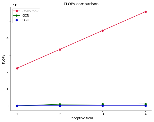
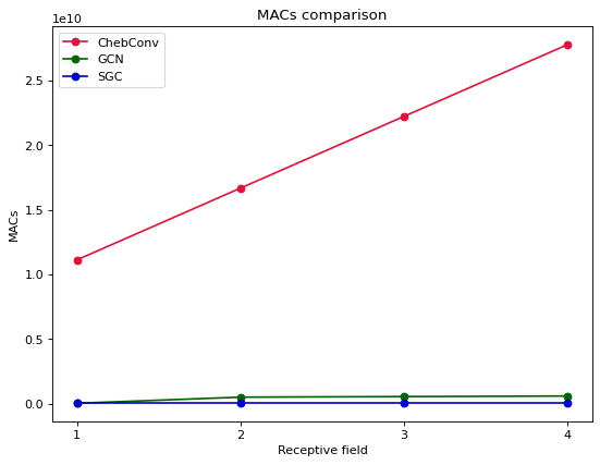
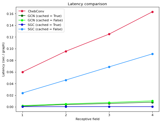
Now, lets plot FLOPs, MACs and latency of ChebConv, GCN, SGC for different receptive fields:

• For all three measures of cost indicators, ChebConv performs the worst out of all model architectures considered.
• For FLOPs and MACs, the difference between GCN and SGC are quite marginal, even as we stack the number of layers.
• For latency, thing are not as simple. When we do not use caching, SGC actually is quite slow compared to GCN. However, SGC becomes very fast with caching enabled, even beating GCNs with caching. Therefore it is strongly advised that we enable caching to True for SGC.

Conclusion

Here, we have compared three important graph convolutional methods, ChebConv, GCN, and SGC. Experiments observing FLOPs, MACs and latency indicate that GCN and SGC are significantly efficient compared to ChebConv, and also the use of caching is critical in latency for SGC models.