Introduction
Semi-supervised learning (SSL) is one of the most widely studied tasks in machine learning. As the ‘supervised’ part of the name suggessts, data instances are accompanied by its labels, which are sereved as the ground-truth. However, ‘semi’ suggests that not all given instance are learned by supervised learning, but rather a (small) portion of it also have access its ground-truth labels by the model. In the context of graph learning, the task of (semi-supervised) node classification is of the main concern for many research papers. The history to solve this task goes quite a way back, one of which is (Zhou et al., 2003), published back in 2003, before the era of machine learning.
In this post, I will revisit this classic method and apply to one of the more modern benchmark datasets, and try to see what analysis can be done to gain some insights.
Setup & Task
One of the main points to consider beforehand is the fact that [1] assumes that the given dataset is not a graph. Rather, it is a ‘typical’ dataset where we are given a bunch of datapoints that can be described as a set of vectors with a fixed dimension, along with a set of class labels. So one of the main concern of the paper is actually the construction of a graph in which the main algorithm will run on. This graph basically constructs a connection (or an edge in graph terms) based on the pairwise similarity between two datapoints. Therefore, the structure of the resulting graph will highlight how much each data have common features in the context of the enitre dataset; a data with a lot of connections will likely to have information shared across many other datapoints.
However, since we are interested in applying the main algorithm in modern graph benchmark datasets, we will skip the graph construction part altogether. Instead, we will use the given graph structure directly, and lets see how it performs.
Main Idea of the algorithm
The algorithm itself is first described as an iterative process. Going a bit formal, let us define some terms here:
- Denote \(n\) as the number of datapoints (which is equal to the number of nodes if we interpret the dataset as a graph).
- As we deal with graph datasets, we can assume that the adjacency matrix \(A \in \mathcal{R}^{n \times n}\) is given. (Separately constructed as an affinity matrix in [1])
- Assume each nodes are assigned to one of \(c\) classes, which we express as a one-hot encoded vector.
- The matrix \(\mathcal{Y} \in \mathcal{R}^{n \times c}\) represents the class information for all nodes in the dataset.
- The task is to generate a good prediction matrix \(\mathcal{F} \in \mathbb{R}^{n \times c}\), where the actual predicted class is considered as the index of the highest value for each row: \(y_i = \text{arg} \max_{j} \mathcal{F}_{ij}\).
Commonly used assumption in SSL
The iteration itself encompasses the philosophy of solving the problem of semi-supervised classification. Naturally, we would like to directly utilize the label information of the nodes that are available (Idea 1). Unfortunately, most of the nodes does not have such access. Semi-supervised (node) classification therefore adopts the following assumption about the dataset (task):
which tends to be effective for quite a lot of cases.
Algorithm
The two ideas (direct loss and similarity assumption) are directly represented in the algorithm, where it can be written as an iterative procedure in the \(t\)-th step:
\[\mathcal{F}(t+1) = \alpha A \mathcal{F}(t) + (1-\alpha)\mathcal{Y}.\]Dissecting each term, we can recover each of the ideas directly. Starting from the second term, \((1-\alpha)\mathcal{Y}\) basically just asserts the label information (at least the available ones) into \(\mathcal{F}(t+1)\) (Idea 1). Now the first term, \(\alpha A \mathcal{F}(t)\), basically reuse the sum (scaled down by \((1-\alpha)\)) of what their neighbor says (Idea 2). Here, we implicitly defined the notion of ‘similar’ in the graph case: Connected nodes are close to each other. This assumption also works well for other graph laerning.
Limit case
The nice thing about this formulation is that, we can directly calculate \(\lim_{t \rightarrow \infty} \mathcal{F}(t)\) analytically. The math itself is also quite straightforward, and the asymptotic result is:
\[\lim_{t \rightarrow \infty} \mathcal{F}(t) = (I - \alpha S)^{-1} Y\]Application to Cora
Cora is perhaps the most used graph benchmark dataset for evaluating on node or edge level tasks (popularized by (Yang et al., 2016)). As mentioned, we will only use the graph structure data as the algorithm does not accept node feature as input.
We will use pytorch and pytorch geometric as our base framework.
import numpy as np
import torch
import os
from torch.nn import functional as F
from torch_geometric.datasets import Planetoid
from torch_geometric.utils import to_dense_adj
import matplotlib.pyplot as plt
from tqdm import tqdm

benchmark = "Cora"
dataset = Planetoid(root="".join([os.getcwd(), "/Cora"]), name="Cora")
data = dataset[0]

device = torch.device("cuda" if torch.cuda.is_available() else "cpu")

data.x = torch.FloatTensor(data.x)
onehot_label = F.one_hot(data.y, num_classes=dataset.num_classes)
onehot_label = onehot_label.float()
x_train = data.x[data.train_mask]  # feature matrix
y_train = onehot_label[data.train_mask]  # node labels
Implementation 1: Explicit iteration
As a first step, we process the data more fit to the algorithm.
A = to_dense_adj(data.edge_index).squeeze_()
D_half = torch.diag((A.sum(dim=1).squeeze_()) ** (-1 / 2), diagonal=0)
S = D_half @ A @ D_half # Normalization according to the paper
blank = torch.Tensor([0.0, 0.0, 0.0, 0.0, 0.0, 0.0, 0.0])
Y = torch.zeros_like(onehot_label) # This is the actual data
for row in range(onehot_label.shape[0]):
    if data.train_mask[row]:
        Y[row] = onehot_label[row] # Masking is needed to ensure only using training data
The implementation can be straightforwardly done by following the paper:
# Custom function to measure the accuracy
def calculate_accuracy(raw_prediction, target) -> float:
    indexed_prediction = torch.argmax(raw_prediction, dim=1)
    indexed_target = torch.argmax(target, dim=1) if target.dim() > 1 else target
    return sum(indexed_prediction == indexed_target).item() / len(indexed_prediction)

# Explicitly define one iteration of the algorithm
def run_one_iteration(F, alpha, S, Y):
    return alpha * torch.mm(S, F) + (1 - alpha) * Y

# Run the whole iteration for a given tot_iteration
def run_explicit_algorithm(alpha, S, Y, tot_iteration, target, mask):
    acc_list = []
    F = Y  # initial iteration
    for _ in tqdm(range(tot_iteration), desc=f"Alpha: {alpha:.1f}"):
        prediction = run_one_iteration(F, alpha, S, Y)
        accuracy = calculate_accuracy(prediction[mask, :], target[mask])
        acc_list.append(accuracy)
        F = prediction  # for the next iteration
    return acc_list

# Run multiple sessions by varying alpha
def experiment_with_alpha(S, Y, tot_iteration, target, mask):
    alpha_list = np.linspace(0.1, 0.9, num=9)
    return [
        run_explicit_algorithm(alpha, S, Y, tot_iteration, target, mask)
        for alpha in alpha_list
    ]

# The results for the whole session is saved in result
tot_iteration = 16
result = experiment_with_alpha(
    S=S,
    Y=Y,
    tot_iteration=tot_iteration,
    target=data.y,
    mask=~data.train_mask,
)
Here, the performance is measured by accuracy (for the test nodes of course).
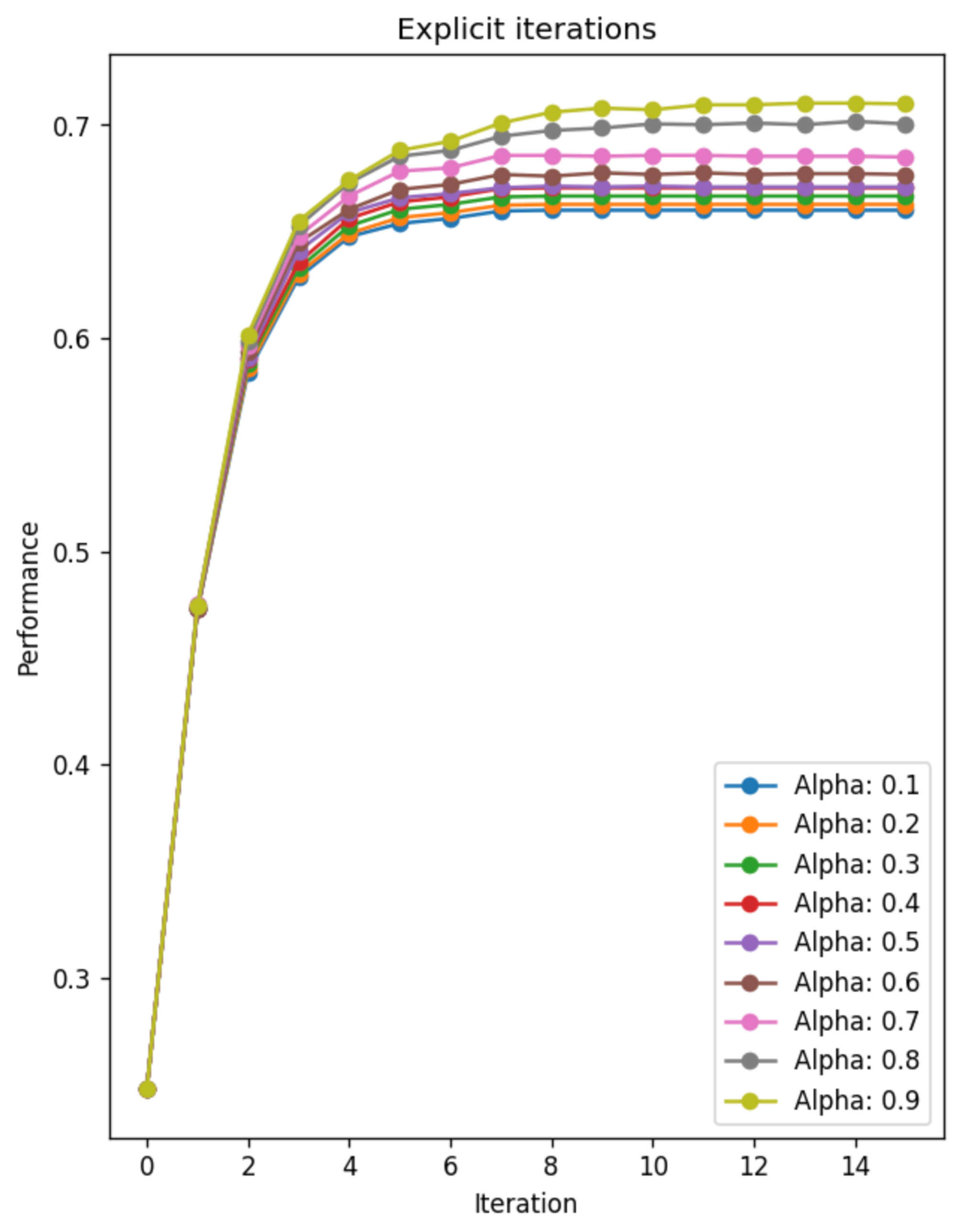
Plotting all experiment sessions in which we perform experiments with different values of alpha:

According to this result, there are some interesting characteristics that we can observe:
- The iteration converges quite fase, and we need ~10 iterations to achieve performance near convergence. We will see this more directly in the next experiment.
- The effect of alpha is quite consistent accros all values: As alpha increases, the model achievec higher performance. The interpretation of this effect is also strightforward: The neighbor information is quite helpful for solving node classification task in Cora, and the given graph structure is nicely aligned with the ‘closeness’ that we discussed earlier. We will also see this effect again in the next experiment.
Implementation 2: Analytic limit solution
Now, we will implement the solution by taking the iteration \(t\) to \(\infty\). This is even more straightfoward:
# Direct calculation of limit solution
def get_prediction_limit(S, Y, alpha) -> torch.Tensor:
    return torch.inverse(torch.eye(W.shape[0]) - alpha * S) @ Y


# Get the performance of the experiment
def perform_experiment_limit(S, Y, alpha, target, mask) -> float:
    raw_prediction = get_prediction_limit(S, Y, alpha)
    return calculate_accuracy(raw_prediction[mask, :], target[mask])

# The experiment is done with various alpha values
performace_list_limit = []
alpha_list = np.linspace(0.1, 0.9, num=9)
for alpha in alpha_list:
    result = perform_experiment_limit(
        S=S, Y=Y, alpha=alpha, target=data.y, mask=~data.train_mask
    )
    performace_list_limit.append(result)
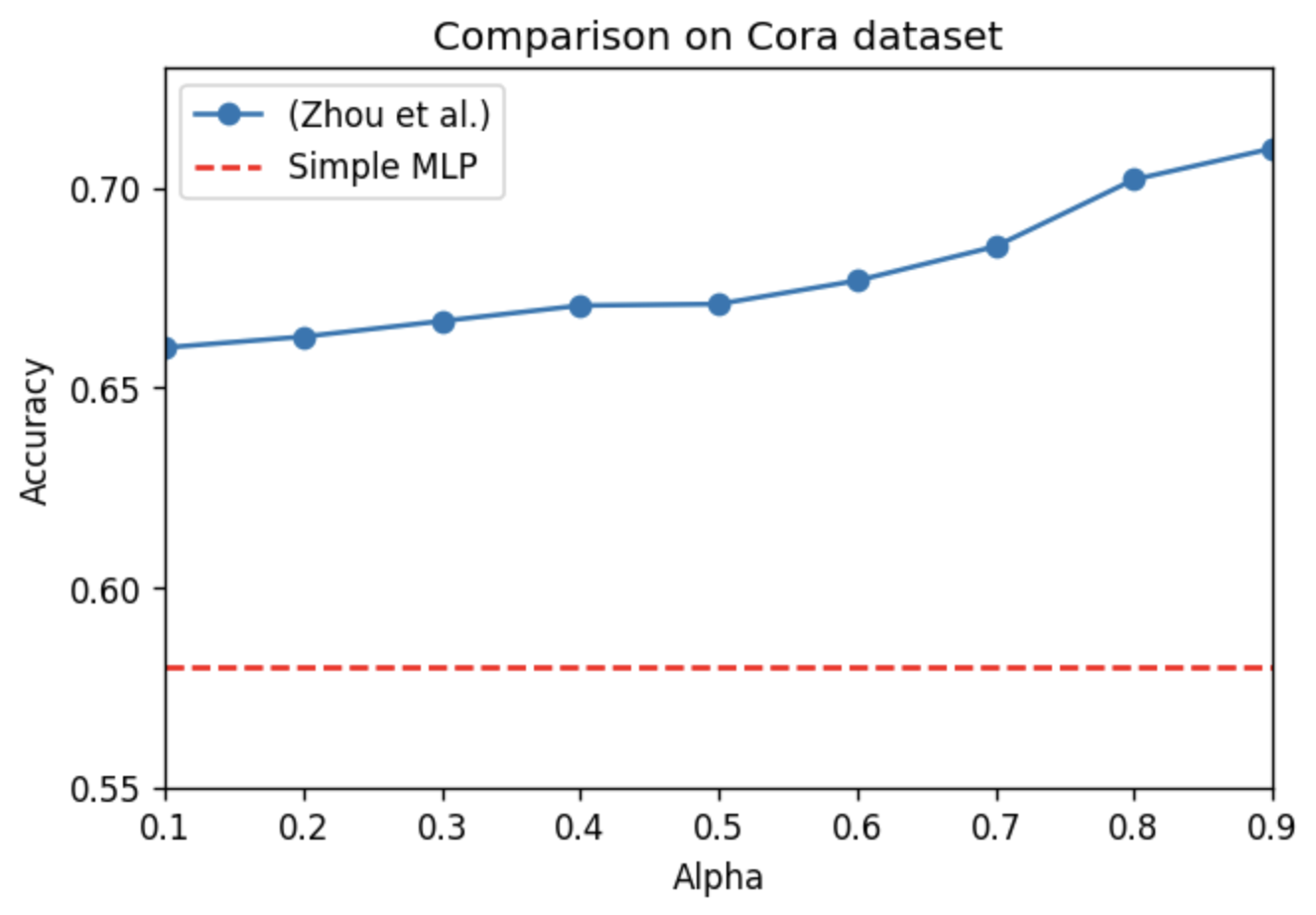
Again, plotting all results of the limit solution version as a plot results in:

From this plot, we also observe some characteristics:
- The effect of alpha is consisent with that of Figure 1.
- The plot also shows the performance of only using the feature information of Cora by training a two-layer MLP model. Although the performance is not that bad (considering only using a part of the model + simple model), (Zhou et al., 2003) still outperforms. This implies that the neighbor information is more vital than the node feature information.
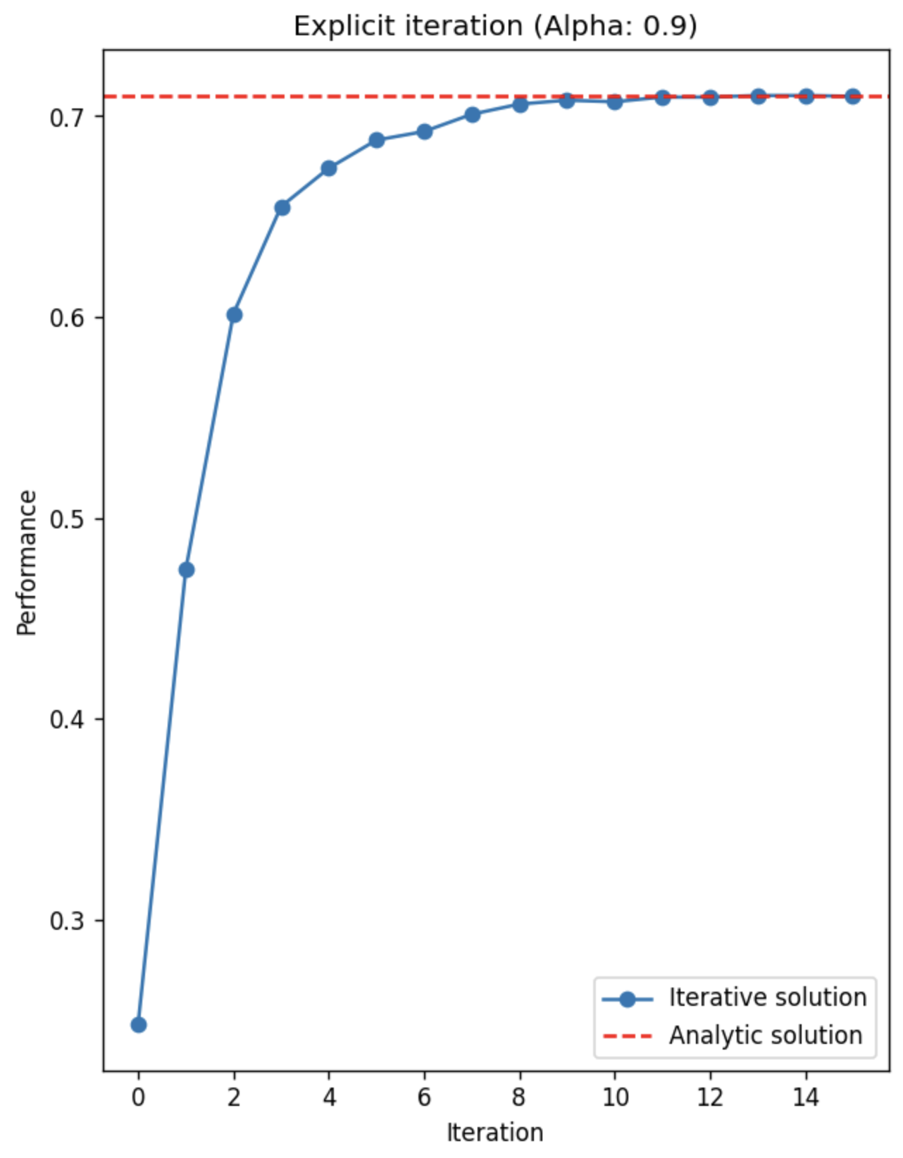
Additionally, we can plot the asymtotic behavior of the iteative algorithm:

As mentioned, the iteration converges quite fast, and achieves the optimal performance near ~10 iterations. However, we need furhter experimental evaluations to see whether this fast convergence is due to the dataset or the algorithm.
Conclusion
In this post, we have revisited the task of semi-supervised node classification. The frequently used benchmark dataset for modern graph learning models, Cora, was tested with a more classical (but insightful) matrix iterative method. Although the algorithm only utilizes the graph information and does not use node feature information, we have seen that the neighbor defined as the graph structure is more critical in soving the task. Perhaps extending to other datasets might reveal to what extent each parts of the dataset (feature vs. structure) affects the performace.